Modifiers¶

In our simple examples so far, we’ve only used two types of modifiers, but HistFactory allows for a handful of modifiers that have proven to be sufficient to model a wide range of uncertainties.

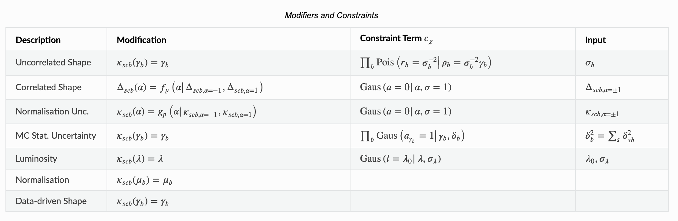
We’ve provided a nice table of Modifiers and Constraints in the introduction of our pyhf documentation to use as reference.

modifiers and constraints

In each of the sections below, we will explore the impact of modifiers on the data.

import pyhf
import ipywidgets as widgets

Unconstrained Normalisation (normfactor)¶

This is a simple scaling of a sample (primarily used for signal strengths). Controlled by a single nuisance parameter.

model = pyhf.Model(
  {
    "channels": [
      {
        "name": "singlechannel",
        "samples": [
          {
            "name": "signal",
            "data": [5.0, 10.0],
            "modifiers": [
              {"name": "mynormfactor", "type": "normfactor", "data": None}
            ]
          }
        ]
      }
    ]
  }, poi_name=None
)

print(f'  aux data: {model.config.auxdata}')
print(f'   nominal: {model.expected_data([1.0])}')
print(f'2x nominal: {model.expected_data([2.0])}')
print(f'3x nominal: {model.expected_data([3.0])}')

@widgets.interact(normfactor=(0, 10, 1))
def interact(normfactor=1):
    print(f'normfactor = {normfactor:2d}: {model.expected_data([normfactor])}')

  aux data: []
   nominal: [ 5. 10.]
2x nominal: [10. 20.]
3x nominal: [15. 30.]

Normalisation Uncertainty (normsys)¶

This is a simple scaling of a sample, but constrained! Controlled by a single nuisance parameter.

model = pyhf.Model(
  {
    "channels": [
      {
        "name": "singlechannel",
        "samples": [
          {
            "name": "signal",
            "data": [5.0, 10.0],
            "modifiers": [
              {"name": "mynormsys", "type": "normsys", "data": {"hi": 0.9, "lo": 1.1}}
            ]
          }
        ]
      }
    ]
  }, poi_name=None
)

print(f'  aux data: {model.config.auxdata}')
print(f'      down: {model.expected_data([-1.0])}')
print(f'   nominal: {model.expected_data([0.0])}')
print(f'        up: {model.expected_data([1.0])}')

@widgets.interact(normsys=(-1, 1, 0.1))
def interact(normsys=0):
    print(f'normsys = {normsys:4.1f}: {model.expected_data([normsys])}')

  aux data: [0.0]
      down: [ 5.5 11.  -1. ]
   nominal: [ 5. 10.  0.]
        up: [4.5 9.  1. ]

What do you think happens if we switch "hi" and "lo"?

Correlated Shape (histosys)¶

A shape uncertainty, but fully correlated across bins. Controlled by a single nuisance parameter.

Unlike most other modifiers, this is an additive effect.

model = pyhf.Model(
  {
    "channels": [
      {
        "name": "singlechannel",
        "samples": [
          {
            "name": "signal",
            "data": [5.0, 10.0],
            "modifiers": [
              {"name": "myhistosys", "type": "histosys", "data": {"hi_data": [15,22], "lo_data": [5,18]}}
            ]
          }
        ]
      }
    ]
  }, poi_name=None
)

print(f'  aux data: {model.config.auxdata}')
print(f'      down: {model.expected_data([-1.0])}')
print(f'   nominal: {model.expected_data([0.0])}')
print(f'        up: {model.expected_data([1.0])}')

@widgets.interact(histosys=(-1, 1, 0.1))
def interact(histosys=0):
    print(f'normsys = {histosys:4.1f}: {model.expected_data([histosys])}')

  aux data: [0.0]
      down: [ 5. 18. -1.]
   nominal: [ 5. 10.  0.]
        up: [15. 22.  1.]

What’s going on with the data? As this is a shape-related uncertainty, we’re providing (absolute) histograms for the modifier to interpolate the up/down variations with respect to the nominal (the sample data).

Uncorrelated Shape (shapesys)¶

A shape uncertainty, but fully uncorrelated across bins. Controlled by \(n\) nuisance parameters (one for each bin).

model = pyhf.Model(
  {
    "channels": [
      {
        "name": "singlechannel",
        "samples": [
          {
            "name": "signal",
            "data": [5.0, 10.0],
            "modifiers": [
              {"name": "myshapesys", "type": "shapesys", "data": [1,4]}
            ]
          }
        ]
      }
    ]
  }, poi_name=None
)

print(f'aux data: {model.config.auxdata}')
print(f'(1x, 1x): {model.expected_data([1.0, 1.0])}')
print(f'(2x, 2x): {model.expected_data([2.0, 2.0])}')
print(f'(3x, 3x): {model.expected_data([3.0, 3.0])}')

@widgets.interact(shapesys_0=(0, 10, 1), shapesys_1=(0, 10, 1))
def interact(shapesys_0=1, shapesys_1=1):
    print(f'shapesys = ({shapesys_0:2d}, {shapesys_1:2d}): {model.expected_data([shapesys_0, shapesys_1])}')

aux data: [25.0, 6.25]
(1x, 1x): [ 5.   10.   25.    6.25]
(2x, 2x): [10.  20.  50.  12.5]
(3x, 3x): [15.   30.   75.   18.75]

Note the differences with histosys. Here, we specify the absolute uncertainty which is fed into the Poisson constraint. This tends to feel more like a bin-by-bin (bin-wise?) constrained normfactor.

MC Statistical Uncertainty (staterror)¶

Bin-wise scale factor. This is used to model the uncertainty in the bins due to Monte Carlo statistics. Controlled by \(n\) nuisance parameters (one for each bin).

In particular, this tends to be correlated across samples as they’re usually modeled by the same MC generator. Unlike shapesys which is constrained by a Poisson, this modifier is constrained by a Gaussian.

model = pyhf.Model(
  {
    "channels": [
      {
        "name": "singlechannel",
        "samples": [
          {
            "name": "signal",
            "data": [5.0, 10.0],
            "modifiers": [
              {"name": "mystaterror", "type": "staterror", "data": [1.0, 2.0]}
            ]
          }
        ]
      }
    ]
  }, poi_name=None
)

print(f'aux data: {model.config.auxdata}')
print(f'(1x, 1x): {model.expected_data([1.0, 1.0])}')
print(f'(2x, 2x): {model.expected_data([2.0, 2.0])}')
print(f'(3x, 3x): {model.expected_data([3.0, 3.0])}')

@widgets.interact(staterror_0=(0, 10, 1), staterror_1=(0, 10, 1))
def interact(staterror_0=1, staterror_1=1):
    print(f'staterror = ({staterror_0:2d}, {staterror_1:2d}): {model.expected_data([staterror_0, staterror_1])}')

aux data: [1.0, 1.0]
(1x, 1x): [ 5. 10.  1.  1.]
(2x, 2x): [10. 20.  2.  2.]
(3x, 3x): [15. 30.  3.  3.]

This looks/feels a lot like shapesys. Is there a difference in the expected data? What happens to the data for the staterror? (Hint: it has to do with the Gaussian constraint.)

Luminosity (lumi)¶

A global scale factor that applies across channel and sample boundaries. Controlled by a single nuisance parameter.

model = pyhf.Model(
  {
    "channels": [
      {
        "name": "singlechannel",
        "samples": [
          {
            "name": "signal",
            "data": [5.0, 10.0],
            "modifiers": [
              {"name": "lumi", "type": "lumi", "data": None}
            ]
          }
        ]
      }
    ],
    "parameters": [{ "name":"lumi", "auxdata":[1.0],"sigmas":[0.017], "bounds":[[0.915,1.085]],"inits":[1.0] }]
  }, poi_name=None
)

print(f'aux data: {model.config.auxdata}')
print(f'(1x, 1x): {model.expected_data([1.0, 1.0])}')
print(f'(2x, 2x): {model.expected_data([2.0, 2.0])}')
print(f'(3x, 3x): {model.expected_data([3.0, 3.0])}')

@widgets.interact(lumi=(0, 10, 1))
def interact(lumi=1):
    print(f'lumi = {lumi:2d}: {model.expected_data([lumi])}')

aux data: [1.0]
(1x, 1x): [ 5. 10.  1.]
(2x, 2x): [10. 20.  2.]
(3x, 3x): [15. 30.  3.]

Data-driven Shape (shapefactor)¶

Bin-wise multiplicative parameters to support data-driven estimation of sample rates (e.g. think of estimating multi-jet backgrounds). Controlled by \(n\) nuisance parameters (one for each bin).

This feels like a bin-wise normfactor.

model = pyhf.Model(
  {
    "channels": [
      {
        "name": "singlechannel",
        "samples": [
          {
            "name": "signal",
            "data": [5.0, 10.0],
            "modifiers": [
              {"name": "myshapefactor", "type": "shapefactor", "data": None}
            ]
          }
        ]
      }
    ]
  }, poi_name=None
)

print(f'aux data: {model.config.auxdata}')
print(f'(1x, 1x): {model.expected_data([1.0, 1.0])}')
print(f'(2x, 2x): {model.expected_data([2.0, 2.0])}')
print(f'(3x, 3x): {model.expected_data([3.0, 3.0])}')

@widgets.interact(shapefactor_0=(0, 10, 1), shapefactor_1=(0, 10, 1))
def interact(shapefactor_0=1, shapefactor_1=1):
    print(f'staterror = ({shapefactor_0:2d}, {shapefactor_1:2d}): {model.expected_data([shapefactor_0, shapefactor_1])}')

aux data: []
(1x, 1x): [ 5. 10.]
(2x, 2x): [10. 20.]
(3x, 3x): [15. 30.]

Correlating Modifiers¶

Like in HistFactory, modifiers are controlled by parameters which are named based on the name you assign to the modifier. Therefore, as long as the modifiers you want to correlate are “mostly” compatible (e.g. same number of nuisance parameters allocated), you can correlate them!

Let’s repeat the normsys example, and through in a histosys on top - both controlled by a single nuisance parameter.

model = pyhf.Model(
  {
    "channels": [
      {
        "name": "singlechannel",
        "samples": [
          {
            "name": "signal",
            "data": [5.0, 10.0],
            "modifiers": [
              {"name": "imshared", "type": "normsys", "data": {"hi": 0.9, "lo": 1.1}},
              {"name": "imshared", "type": "histosys", "data": {"hi_data": [15,22], "lo_data": [5,18]}}
            ]
          }
        ]
      }
    ]
  }, poi_name=None
)

print(f'  aux data: {model.config.auxdata}')
print(f'      down: {model.expected_data([-1.0])}')
print(f'   nominal: {model.expected_data([0.0])}')
print(f'        up: {model.expected_data([1.0])}')

@widgets.interact(imshared=(-1, 1, 0.1))
def interact(imshared=0):
    print(f'imshared = {imshared:4.1f}: {model.expected_data([imshared])}')

  aux data: [0.0]
      down: [ 5.5 19.8 -1. ]
   nominal: [ 5. 10.  0.]
        up: [13.5 19.8  1. ]

Isn’t that crazy? We’re seeing the impact of a multiplicative bin-wise correlated shape modification convoluted with an additive normalization uncertainty - both constrained by a Gaussian.

ATLAS Exotics + SUSY Workshop 2020 pyhf Tutorial