HistFactory¶

pyhf stands for python-based HistFactory.

It’s a tool for statistical analysis of data in High Energy Physics.

In this chapter, we will cover

What HistFactory is in general
What pyhf is specifically (and what it is not)

Statistical Analysis¶

We divide analyses into the type of fit being performed:

unbinned analysis (based on individual observed events)
binned analyses (based on aggregation of events)

Like HistFactory, pyhf does not work with unbinned analyses. These will not be covered in the tutorial.

So what uses HistFactory?

TRexFitter
WSMaker
HistFitter

Most everyone in SUSY and Exotics who performs an asymptotic fit as part of their analysis is likely using HistFactory!

Why Binned?¶

Most likely, one performs a binned analysis if no functional form of the p.d.f. is known. Instead, you make approximations (re: educated guesses) as to this functional form through histograms.

What is a histogram? Fundamentally, a histogram is a tool to bookkeep arrays of numbers:

binning
counts
errors

Beyond that, it contains lots of other magic ingredients to make them more user-friendly for common operations (addition, division, etc…).

What are the ingredients?¶

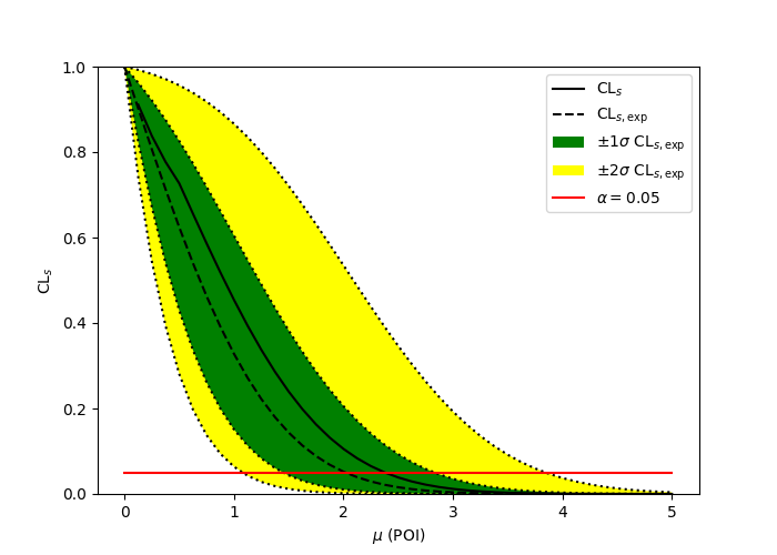
Once you have a model, you can perform inference such as

exclusion fit (upper limits)
discovery fit (lower limits)
measurement (two-sided intervals)
parameter scans
impact plots
pull plots
…

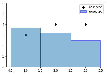
Let’s make up some samples and histograms to go along with it to understand what’s going on. Suppose we have an analysis with expected event rate \(\lambda\) and measurements \(n\). For this incredibly simple case, the overall probability of the full experiment is the joint probability of each bin:

\[ p(n|\lambda) = \prod_{\mathrm{bin}\ b} \mathrm{Pois}(n_b | \lambda_b) \]

Why Poisson? This is a counting experiment after all. A region we want to model will then just be a series of Poissons.

import matplotlib.pyplot as plt

bins = [1,2,3]
observed = [3, 4, 4]
expected_yields = [3.7, 3.2, 2.5]

fig, ax = plt.subplots()
ax.bar(bins, expected_yields, 1.0, label=r'expected', edgecolor='blue', alpha=0.5)
ax.scatter(bins, [3, 4, 4], color='black', label='observed')
ax.set_ylim(0,6)
ax.legend();

However, we don’t always often have just a single (MC) sample, and \(\lambda\) is often the sum of multiple sample yields

\[ \lambda = \sum_{\mathrm{sample}\ s} \lambda_s \]

A typical case might be multiple (sub)dominant backgrounds or having a model where the observed events are described by a signal + background p.d.f. Then the p.d.f. might look like

\[ p(n|\lambda) = \prod_{\mathrm{bin}\ b} \mathrm{Pois}(n_b | \lambda_b) \qquad \lambda_b = \sum_{\mathrm{sample}\ s} \lambda_{bs} \]

bins = [1,2,3]
observed = [3, 4, 4]
background = [3.0, 1.5, 1.0]
signal = [0.7, 1.7, 1.5]

fig, ax = plt.subplots()
ax.bar(bins, background, 1.0, label=r'$t\bar{t}$', edgecolor='red', alpha=0.5)
ax.bar(bins, signal, 1.0, label=r'signal', edgecolor='blue', bottom=background, alpha=0.5)
ax.scatter(bins, [3, 4, 4], color='black', label='observed')
ax.set_ylim(0,6)
ax.legend();

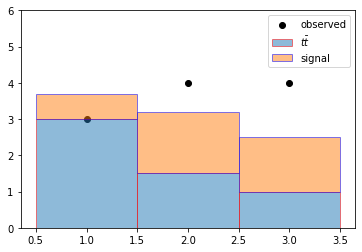
Already, you can see the p.d.f. for this simple case starts expanding to be a little bit more generic, and a little bit more flexible. Now we want to incorporate when the expected yields for signal and backgrounds depend on some parameters, perhaps how we applied calibrations to some objects, or how we configured our Monte-Carlo generators, etc…

Suppose we wanted a \(\mu_s\) that is a normalization factor scaling up (or down!) the sample. For example, if we want to parametrize the signal strength (without changing background). So \(\lambda\) becomes a function of \(\theta = \{\mu\}\) (a set of the parameters that determine the expected event rate), then our p.d.f. expands to be

\[ p(n|\lambda(\mu)) = \prod_{\mathrm{bin}\ b} \mathrm{Pois}(n_b | \lambda_b(\theta)) \qquad \lambda_b(\theta) = \sum_{\mathrm{sample}\ s} \lambda_{bs}(\theta) \]

where \(\mu_{\mathrm{background}} = 1\)

import ipywidgets as widgets

@widgets.interact(mu=(0, 5, 0.1))
def draw_plot(mu=1):
    bins = [1,2,3]
    observed = [3, 4, 4]
    background = [3.0, 1.5, 1.0]
    signal = [i*mu for i in [0.7, 1.7, 1.5]]

    print(f'signal: {signal}')
    print(f'background: {background}')
    print(f'observed: {observed}\n')
    
    fig, ax = plt.subplots()
    ax.bar(bins, background, 1.0, label=r'$t\bar{t}$', edgecolor='red', alpha=0.5)
    ax.bar(bins, signal, 1.0, label=r'signal', edgecolor='blue', bottom=background, alpha=0.5)
    ax.scatter(bins, [3, 4, 4], color='black', label='observed')
    ax.set_ylim(0,6)
    ax.legend();

One final thing to finish our build up of a simplified p.d.f. is about auxiliary measurements. What we mean is that perhaps the background sample is modeled by some normalization parameter, but we’ve also performed additional measurements in a separate analysis that constraints the parametrization (e.g. Jet Energy Scale) so we have stronger confidence that the true parameter is within a certain range.

For some parameters in a statistical model, all we have to infer its values is the given analysis. These parameters are unconstrained (\(\eta\)):

\[ p(n | \lambda(\theta)) \]

For many parameters, we have the auxiliary data (\(a\)) given as an auxiliary measurement which is added to the main p.d.f.. These parameters are constrained (\(\chi\)).

\[ p_\chi(a | \chi) \]

where \(\theta = \{\eta, \chi\}\). This constraining function can generally be anything, but most of the time in HistFactory - it’s a Gaussian or a Poisson. The p.d.f. expands to be

\[ p(n,a|\lambda(\theta)) = \prod_{\mathrm{bin}\ b} \mathrm{Pois}(n_b | \lambda_b(\theta)) \prod_{\mathrm{constraint}\ \chi} p_\chi(a_\chi | \chi) \qquad \lambda_b(\theta) = \sum_{\mathrm{sample}\ s} \lambda_{bs}(\theta) \]

For this simple example, let’s consider a Gaussian centered at \(\mu=0\) with \(\sigma=1\) for constraining the normalization on the background where an up-variation (\(\mu_b = +1\)) scales by 1.3, and a down-variation (\(\mu_b = -1\)) scales by 0.8.

import numpy as np
from scipy.stats import norm

def gaussian_constraint(mu_b=0.0):
    return norm.pdf(mu_b, loc=0.0, scale=1.0)

# interpolating
def interpolate(down,nom,up,alpha):
    if alpha >= 0:
        return (up-nom)*alpha + 1
    else:
        return 1 - (down-nom)*alpha
    
@widgets.interact(mu=(0, 5, 0.1), mu_b=(-1, 1, 0.1))
def draw_plot(mu=1, mu_b=0):
    bins = [1,2,3]
    observed = [3, 4, 4]
    background = [i*interpolate(0.8, 1.0, 1.3, mu_b) for i in [3.0, 1.5, 1.0]]
    signal = [i*mu for i in [0.7, 1.7, 1.5]]

    print(f'signal: {signal}')
    print(f'background: {background}')
    print(f'observed: {observed}')
    print(f'likelihood scaled by: {gaussian_constraint(mu_b)/gaussian_constraint(0.0)}\n')
    
    fig, ax = plt.subplots()
    ax.bar(bins, background, 1.0, label=r'$t\bar{t}$', edgecolor='red', alpha=0.5)
    ax.bar(bins, signal, 1.0, label=r'signal', edgecolor='blue', bottom=background, alpha=0.5)
    ax.scatter(bins, [3, 4, 4], color='black', label='observed')
    ax.set_ylim(0,6)
    ax.legend();

But that’s not all! Notice that all along, we’ve been only discussing a single “channel” with 3 bins. The statistical analysis being studied might involve multiple channels corresponding to different signal regions and control regions. Therefore, we compute the likelihood as

\[ p_\text{main} = p_\text{channel1} * p_\text{channel2} * p_\text{channel3} \cdots \]

So in fact, we can then expand out the likelihood definition further

\[ p(n,a|\theta) = \underbrace{\prod_{\mathrm{channel}\ c}\prod_{\mathrm{bin}\ b} \mathrm{Pois}(n_{cb} | \lambda_{cb}(\theta))}_{\text{main}} \underbrace{\prod_{\mathrm{constraint}\ \chi} p_\chi(a_\chi | \chi)}_{\text{auxiliary}} \qquad \lambda_{cb}(\theta) = \sum_{\mathrm{sample}\ s} \lambda_{cbs}(\theta) \]

As you can see, this is sort of a bookkeeping problem. We have two pieces of this likelihood:

our main model, which consists of
- several channels (regions, histograms, etc), where
- each channel is a set of simultaneous Poissons measuring the bin count against an expected value, where
- the expected value is the sum of various samples, where
- each samples expected value can be a function of parameters (or modifiers)
the constraint model, which consists of
- several auxiliary measurements, where
- each measurement comes with auxiliary data

It should be clear by now that this is quite a lot of pieces to keep track of. This is where HistFactory comes in to play. Using HistFactory, we can

describe observed event rates and expected event rates
use well-defined modifiers to express parameterizations of the expected event rates
use well-defined interpolation mechanisms to derive expected event rates (if needed)
automatically handle auxiliary measurements / additional constraint terms

Note: if you’re curious about interpolation and interesting challenges, see the next chapter.

pyhf¶

Up to about 2 years ago, HistFactory was only implemented using ROOT, RooStats, RooFit (+ minuit). pyhf provides two separate pieces:

a schema for serializing the HistFactory workspace in plain-text formats, such as JSON
a toolkit that interacts and manipulates the HistFactory workspaces

Why is this crucial? HistFactory in ROOT is a combination of loosely-linked XML+ROOT files

XML for structure
ROOT for storing data

These would then be processed through a hist2workspace command to get the ROOT Workspace that RooStats/RooFit use. As an example, let’s look at the provided multichannel HistFactory XML+ROOT as part of this tutorial:

!ls -lhR data/multichannel_histfactory

data/multichannel_histfactory:
total 8.0K
drwxr-xr-x 2 runner docker 4.0K Sep 25 14:02 config
drwxr-xr-x 2 runner docker 4.0K Sep 25 14:02 data

data/multichannel_histfactory/config:
total 20K
-rw-r--r-- 1 runner docker 6.4K Sep 25 14:02 HistFactorySchema.dtd
-rw-r--r-- 1 runner docker  906 Sep 25 14:02 example.xml
-rw-r--r-- 1 runner docker  974 Sep 25 14:02 example_control.xml
-rw-r--r-- 1 runner docker 1.1K Sep 25 14:02 example_signal.xml

data/multichannel_histfactory/data:
total 8.0K
-rw-r--r-- 1 runner docker 5.9K Sep 25 14:02 data.root

Here, we have two folders:

config which provides
- the XML HistFactory schema HistFactorySchema.dtd
- a top-level example.xml
- signal region and control region structures
data which provides the stored histograms in data.root

Let’s just look at the XML structure for now. What does the top-level look like?

!cat -n data/multichannel_histfactory/config/example.xml

<!--
//============================================================================
// Name        : example.xml
//============================================================================
-->

<!--
   Top-level configuration,  details for the example channel are in example_channel.xml.
   This is the input file to the executable.

   Note: Config.dtd needs to be accessible.  It can be found in ROOT release area.
   The file system path is relative to location of this XML file, not the executable.
-->

<!DOCTYPE Combination  SYSTEM 'HistFactorySchema.dtd'>

<Combination OutputFilePrefix="./results/example">
 <Input>./config/example_signal.xml</Input>
 <Input>./config/example_control.xml</Input>
 <Measurement Name="GaussExample" Lumi="1." LumiRelErr="0.1" ExportOnly="True">
   <POI>SigXsecOverSM</POI>
   <ParamSetting Const="True">Lumi</ParamSetting>
 </Measurement>
</Combination>

This top-level specifies:

15: the HistFactory XML schema
17: the workspace definition
18,19: channel definitions (links to other files)
20: a measurement GaussExample with specifications for luminosity, the parameter of interest, and setting lumi constant

What does the signal region look like?

!cat -n data/multichannel_histfactory/config/example_signal.xml

<!--
   Single channel configuration exampple.
   The top level configuration XML is example.xml

   NormalizedByTheory should be "True" (not "TRUE" or "true") for all non-data-driven backgrounds.

   If you comment or remove the <Data> tag then it will use the expected data.

   Histogram inputs should be in pb and in top-level xml the lumi should be in 1/pb
   (The important thing is that they match... fb and 1/fb is also ok)

   Note: Config.dtd needs to be accessible.  It can be found in ROOT release area.
   The file system path is relative to location of this XML file, not the executable.
-->

<!DOCTYPE Channel  SYSTEM 'HistFactorySchema.dtd'>

<Channel Name="channel1" InputFile="./data/data.root" >
 <Data HistoName="signal_data" HistoPath="" />
 <Sample Name="signal" HistoPath="" HistoName="signal_signal">
   <NormFactor Name="SigXsecOverSM" Val="1" Low="0." High="10."  />
 </Sample>
 <Sample Name="bkg" HistoPath="" NormalizeByTheory="True" HistoName="signal_bkg">
   <ShapeSys Name="uncorrshape_signal" HistoName="signal_bkgerr" ConstraintType="Poisson"/>
 </Sample>
</Channel>

This signal region specifies:

16: the HistFactory XML schema
18: the channel definition along with the path to the file for where the data for this channel is stored
19: where the expected event rate (data) for this channel is located
20, 23: sample definitions for signal and bkg with each sample expected event rate stored under HistoName in the corresponding ROOT file
21: a parameter SigXsecOverSM which is an unconstrained normalization factor
24: a parameter uncorrshape_signal which is a Poisson-constrained shape systematic, with the corresponding auxiliary data stored under HistoName in the corresponding ROOT file

As you can see, this works fine. It’s a little bulky, and a lot of loosely-tied information, but this fulls specifies the HistFactory model we’ve discussed so far.

In the next chapter, we’ll learn how to use pyhf to convert to the HistFactory JSON representation.

ATLAS Exotics + SUSY Workshop 2020 pyhf Tutorial

HistFactory¶

Statistical Analysis¶

Why Binned?¶

What are the ingredients?¶

pyhf¶