Model Inference
Inference using pyhf Python API
import pyhf
import json
with open("data/2-bin_1-channel.json") as serialized:
  spec = json.load(serialized)

workspace = pyhf.Workspace(spec)
model = workspace.model(poi_name="mu")
pars = model.config.suggested_init()
data = workspace.data(model)
Creating the log-likelihood conditioned on the data $\( L(\vec{\theta}|\vec{x}) = k \cdot p(\vec{x} | \vec{\theta}) \)$
model.logpdf(pars, data)
array([-12.58363315])
moar inference
bestfit_pars, twice_nll = pyhf.infer.mle.fit(data, model, return_fitted_val=True)
print(bestfit_pars)
[1.72986288e-04 1.00000157e+00 9.99966590e-01]
objective function is twice the negative log-likelihood
-2 * model.logpdf(bestfit_pars, data) == twice_nll
array([ True])
Hypothesis Testing
Very often in physics analyses we want to compute the \(\mathrm{CL}_{s}\) — a modified pseudo-frequentist \(p\)-value. We can use the API that pyhf provides for hypothesis testing to compute the expected and observed \(\mathrm{CL}_{s}\).
test_mu = 1.0
CLs_obs, CLs_exp = pyhf.infer.hypotest(test_mu, data, model, return_expected=True)
print('Observed: {}, Expected: {}'.format(CLs_obs, CLs_exp))
Observed: [0.35998456], Expected: [0.35998495]
As a quick aside, remembering that $\( \mathrm{CL}_{s} = \frac{\mathrm{CL}_{s+b}}{\mathrm{CL}_{b}} = \frac{p_{s+b}}{1-p_{b}} \)$
CLs_obs, p_values = pyhf.infer.hypotest(test_mu, data, model, return_tail_probs=True)
print('Observed CL_s: {}, CL_sb: {}, CL_b: {}'.format(CLs_obs, p_values[0], p_values[1]))
Observed CL_s: [0.35998456], CL_sb: [0.17999205], CL_b: [0.49999935]
we can explicitly check pyhf with
assert CLs_obs == p_values[0]/p_values[1]
We often are intersted in computing a band of expected \(\mathrm{CL}_{s}\) values (the “Brazil band”)
import numpy as np

CLs_obs, CLs_exp_band = pyhf.infer.hypotest(test_mu, data, model, return_expected_set=True)
print('Observed CL_s: {}\n'.format(CLs_obs))
for p_value, n_sigma in enumerate(np.arange(-2,3)):
    print('Expected CL_s{}: {}'.format('      ' if n_sigma==0 else '({} σ)'.format(n_sigma),CLs_exp_band[p_value]))
Observed CL_s: [0.35998456]

Expected CL_s(-2 σ): [0.07807428]
Expected CL_s(-1 σ): [0.17472572]
Expected CL_s      : [0.35998495]
Expected CL_s(1 σ): [0.63435682]
Expected CL_s(2 σ): [0.8809947]
We can scan across test values of our POI (\(\mu\)) to perform hypothesis testing for our model
results = []
poi_vals = np.linspace(0,5,41)
for test_poi in poi_vals:
    results.append(
        pyhf.infer.hypotest(test_poi, data, model, return_expected_set=True)
    )
and then invert those hypothesis tests to set upper limits on the model parameters
obs = [cls_vals[0][0] for cls_vals in results]
exp = [cls_vals[1][2][0] for cls_vals in results]

alpha = 0.05
cls_limit = (1.-alpha)*100

print(f"{cls_limit}% CLs Upper Limit (observed): µ = {np.interp(0.05, obs[::-1], poi_vals[::-1]):0.3}")
print(f"{cls_limit}% CLs Upper Limit (expected): µ = {np.interp(0.05, exp[::-1], poi_vals[::-1]):0.3}")
95.0% CLs Upper Limit (observed): µ = 2.12
95.0% CLs Upper Limit (expected): µ = 2.12
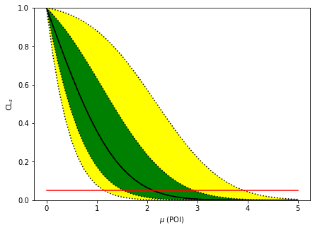
Visualization
We can visualize this by plotting the observed and expected results (the “Brazil band”)
import matplotlib.pyplot as plt
import pyhf.contrib.viz.brazil
fig, ax = plt.subplots(1,1)
fig.set_size_inches(7, 5)

ax.set_xlabel(r"$\mu$ (POI)")
ax.set_ylabel(r"$\mathrm{CL}_{s}$")

pyhf.contrib.viz.brazil.plot_results(ax, poi_vals, results)