Model-Independent Upper Limits¶

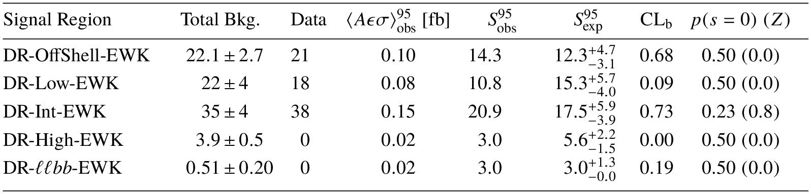
This section is aiming to cover some common concepts about (model-independent) upper limits. While it won’t necessarily be exhaustive, the aim is to summarize the current working knowledge of how High Energy Physics experiments such as ATLAS produce tables such as Table 20 from the Supersymmetry Electroweak 2-lepton, 2-jet analysis (SUSY-2018-05):

Here, the ATLAS collaboration provided some text describing each of the individual columns. How does that translate to statistical fits and pyhf? Let’s explore below. We will use the public probability models from the analysis published on HEPData entry.

Downloading the public probability models¶

First, we’ll use pyhf.contrib to download the models from HEPData:

Then use Python’s tarfile (part of standard library) to extract out the JSONs:

and then build our workspace for a particular signal region DR-Int-EWK:

Understanding expected and observed events¶

The background estimate(s) in the signal region(s) are obtained from the background-only fit to control region(s) extrapolated to the signal region(s).

This number, combined with the number of observed events in the signal region, allows us to redo the limit-setting or $p$-value determination without the public probability models.

For the uncertainties on the background estimate(s) in the signal region(s), they’re symmetric and calculated through standard error propagation described below.

Observed Events¶

The observed events are just ws.data(model) which we will call data. These are ordered in the same way as the ordering of the channels in the model (model.config.channels):

Expected Events¶

The expected events are determined from a background-only fit. This is done by fixing the parameter of interest (i.e. for a search the non-SM signal strength) to zero. This fit will give us the fitted parameters $\hat{\theta}$. From this, we can print out the expected background events in each channel after this fit:

The uncertainty on the total background (expected event rate) is done by linearly propagating errors on parameters using the covariance matrix from a fit result. The error is calculated in the same way that ROOT’s RooAbsReal::getPropagatedError() calculates it. It is summarized as follows

where

with $f(x)$ the probability model and $\mathrm{d}\mathbf{a}$ the vector of one-sigma uncertainties of all fit parameters taken from the fit result and $\mathrm{Corr}(\mathbf{a},\mathbf{a}')$ the correlation matrix from the fit result.

References:

• Statistical Error Propagation (J. Phys. Chem. A 2001, 105, 15, 3917–3921)

• root-project/root#13404

Note: be aware that some definitions of error propagation use covariance and some use correlation. You can translate between the two, turning covariance into correlation by multiplying by $\partial a$ on both sides. If one uses covariance, you’ll need information about the derivatives (e.g. through auto-differentiation).

This could be done with a for-loop like so:

up_yields = []
dn_yields = []
for i, variation in enumerate(uncrt_bonly):
    varied_up_pars = pars_bonly[:] # copy
    varied_up_pars[i] += variation
    
    varied_dn_pars = pars_bonly[:] # copy
    varied_dn_pars[i] -= variation

    up_yields.append(model.expected_actualdata(varied_up_pars))
    dn_yields.append(model.expected_actualdata(varied_dn_pars))

which gives us the up/down variations on the yields for each systematic. However, we’ll batch this calculation to calculate all yield variations simultaneously. To do this, we set up our model to allow for batching.

Then we calculate the up_yields and dn_yields which are used to calculate the $F_\mathbf{a}(x)$ term above, denoted as variations:

Now we can calculate $\mathrm{error}^2(x)$:

Taking the square root will give us the propagated uncertainty on the yields per-region for the background-only fit. We can update our table:

Understanding visible cross-section¶

See ATL-PHYS-PUB-2022-017 for descriptions of detector efficiency and selection acceptance.

Production cross section upper limits is another way of saying model-dependent limits. Without the detector efficiency (but keeping selection acceptance), the term visible cross section upper limits is used.

For upper limits on numbers of events (and the corresponding cross section), after detector efficiency and selection acceptance effects, the term model independent upper limits is used. These upper limits are typically free from assumptions about the acceptance and efficiency of any model (and are model independent in that sense), but they do make the assumption that signal contamination in control regions is negligible.

Model-independent Upper Limits¶

Model-independent upper limits (UL) at the 95% confidence level (CL) on the number of beyond the SM (BSM) events for each signal region are derived using the $\mathrm{CL}_\mathrm{s}$ prescription (DOI: Read (2002)) and neglecting any possible contamination in the control regions.

To obtain the 95% CL model-independent UL / discovery $p_0$-value, the fit in the signal region proceeds in the same way as the background-only fit, except that an additional parameter for the non-SM signal strength, constrained to be non-negative, is fit.

When calculating $S^{95}_\mathrm{obs}$ (also for expected) it is typical to inject a test signal (all expected event rates equal to unity) which means for this signal, we’re assuming $A\times\varepsilon\times\sigma\times\mathcal{L}=1$. As $S^{95}_\mathrm{obs}$ is an upper limit on $\mu$ for this test signal, normalizing this by the integrated luminosity of the data sample allows us to interpret as upper limits on the visible (BSM) cross-section, $\langle A\varepsilon\sigma\rangle_\mathrm{obs}^{95}$. This is defined as the product of acceptance, reconstruction efficiency and production cross-section.

Remember that we often call this the visible cross-section, where cross-section is $\sigma$ and the visible cross-section is $A\times\varepsilon\times\sigma$. This is called a model independent limit as we do not have a specific model in mind (hence the test signal). We don’t have specific values for selection acceptance $A$, detector efficiency $\varepsilon$, or signal model cross-section $\sigma$, so we can only say something about the product. If we have a specific signal model with $A\varepsilon\sigma$ that gives us a cross-section higher than the limit on the visible cross-section, we should be able to see that signal in the analysis.

Discovery $p$-values¶

The significance of an excess can be quantified by the probability ($p_0$) that a background-only experiment is more signal-like than observed. The last two columns indicate the $\mathrm{CL}_\mathrm{b}$ value and the discovery $p$-value ($p(s)=0$) with the corresponding gaussian significance ($Z$$\,$).

These two numbers provide information about the compatibility of the observed data with a background-only hypothesis, albeit with different test statistics $q$. The $q_\mu$ (or $\tilde{q}_\mu$) test statistic is optimized for hypothesis-testing the signal+background hypothesis. The $q_0$ test statistic is optimized for hypothesis-testing the background-only hypothesis.

From Equation 52 in arXiv:1503.07622:

• for $p_\mu$: the null hypothesis is signal at a rate $\mu' < \mu$ and the alternative hypothesis is signal at a rate of $\mu$

• for $p_0$: the null hypothesis is background-only (b) and alternative hypothesis is signal+background (s+b)

For these hypotheses, we find that the $p$-values are

and

Note that the same $q_\mathrm{obs}$ value is used to determine $p_\mu$ and $p_b$.

$p_\mu$ (and $\mathrm{CL}_\mathrm{b}$)¶

$\mathrm{CL}_\mathrm{b}$ provides a measure of compatibility of the observed data with the 95% CL signal strength hypothesis relative to fluctuations of the background. $\mathrm{CL}_\mathrm{b}$ is evaluating $p_\mu$ in the case where $\mu'=0$ and $\mu=\mu_{95}$ (the fitted $\mu$ at the upper limit $S^{95}_\mathrm{obs}$). This is saying that the tested $\mu$ is the 95% CL signal strength ($\mu_{95}$) but the assumed true $\mu$ is the background-only hypothesis ($\mu'=0$):

Note that this calculation depends on the value of $\mu$ at the fitted upper limit $S^{95}_\mathrm{obs}$. You get a small $\mathrm{CL}_\mathrm{b}$ if you have a downward fluctuation in observed data relative to your signal+background hypothesis, preventing you from excluding your signal erroneously if you “shouldn’t be able to” when using $\mathrm{CL}_\mathrm{s}$ (since you would be dividing by a small number). See the paragraph above plot on page two in this document.

$p_0$¶

$p(s)=0$ measures compatibility of the observed data with the background-only (zero signal strength) hypothesis relative to fluctuations of the background. Larger values indicate greater relative compatibility. $p(s)=0$ is not calculated in signal regions with a deficit with respect to the nominal background prediction.

This is saying that the tested $\mu$ is the background-only hypothesis ($\mu=\mu'=0$) and the assumed true $\mu$ is the background-only hypothesis:

Relationship to $\mathrm{CL}_\mathrm{s}$¶

This will be covered through a learn notebook, which will be added as part of scikit-hep/pyhf#2274.

Calculating the $p$-values¶

Armed with all of this knowledge, we can first calculate the discovery $p$-value evaluated at $\mu=\mu'=0$, as well as convert this to a Z-score assuming a “standard” Normal distribution:

And similarly, we can extract $\mathrm{CL}_\mathrm{b}$ by evaluating at $\mu=\mu_{95}^\mathrm{obs}$ :

Making the table¶

Now that we have all of our numbers, we can make the table for the discovery region DRInt_cuts. We’ll get the corresponding index of the channel so we can extract out the total background and uncertainty estimates from above.

• Will Buttinger

• Jonathan Long

• Zach Marshall

• Alex Read

• Sarah Williams